
Authors: Bryant, A., Freilich, B., & Papova, A.
Synopsis: Microsoft Excel can assist with organizing your neuropsychological test data and can be used to streamline your scoring and report writing.
Author Disclosures: Nothing to disclose.
Overall Description: Microsoft Excel is an efficient and reliable tool for organizing, analyzing, and presenting neuropsychological test data. It allows for easy scoring of tests, reducing the risk of human error. Normative data can be easily stored and accessed in Excel, and its formulas can be used to compare a patient’s performance to these norms. Additionally, Excel can be used to create clear and concise data summary tables for inclusion in neuropsychological reports. By cutting down on the time taken for scoring and report writing, clinicians can focus on other important activities or see more testing cases.
Tutorials/Case Study Examples:
Excel can assist with scoring
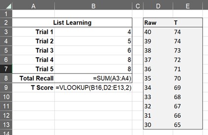
Formulas in Excel can be simple and save you time! For example, a simple SUM formula can total correct responses on a list-learning task:
- Enter the raw scores for each trial in cells B3-B7
- In cell B8 (where the total correct will appear), enter the formula =SUM(B3:B7) and press Enter.
Formulas can get more complex, and be even more useful. For example, the VLOOKUP formula can pull in the appropriate normative score for total correct as calculated in call B8 from the above example.
- Enter normative table in cells D3:E13 (raw score down column D, T score down column E).
- Click on the cell where you want to look up the normative score (e.g., cell B9)
- Enter the formula =VLOOKUP(B8,D2:E13,2) and press Enter.
Some helpful tricks:
- Instead of using Excel formulas to look up norms and quantify performance (see above), one can simply import scores into Excel from other sources.
- For example, many tests use scoring programs (e.g., Pearson QGlobal) that automatically convert raw scores into standard scores. Why not copy these data (either directly from the program or from a scoring report) and paste them into an Excel spreadsheet where you can easily link them to your own data tables?
- Alternatively, did you know that the Microsoft Office/365 smartphone app has a function in which you can take a picture of a table (e.g., from a scoring report) and import it to an Excel file? Just be careful not to scan any personal health information (unless you are using a HIPAA compliant smartphone)!
Excel can assist with creating data tables
First, create a new Excel workbook or open the workbook you already have and want to edit. Decide how you want to organize your data table. For example, you can create columns for the name of the Measure, various Scores (raw, standard, scaled, T, z, percentile), Interpretation (for an interpretive label), Interval Change in case of re-evaluation, and Notes for anything that might’ve happened during that particular test. For rows, decide how you want to organize your measures. For example, consider organizing by cognitive domain and listing the measures you commonly use within each domain. Not every score has to be listed, but make sure to create rows for all of the variables you use (subscales, trials, etc.).
Excel makes it easy to automatically calculate percentiles from normal distributions. Please note that from here on, formulas will be provided which reference specific cells within the document. Whenever you see a letter and number combination, such as D4, it is talking about the value in the cell in column D row 4. Please change these values to the actual cells you will be using in your document, they are just provided as examples. Use the following formulas to obtain percentiles based on scores:
- For standard scores, enter the following formula into the cell. If the standard score cell for that measure is not blank, it will designate a percentile based on a normal distribution with a mean of 100 and standard deviation of 15.
- For scaled scores, use: =IF(ISBLANK(E4),””,NORMDIST(E4,10,3,TRUE)*100)
- For T scores, use: =IF(ISBLANK(G4),””,NORMDIST(G4,50,10,TRUE)*100)
- For z-scores, use: =IF(ISBLANK(F4),””,NORMSDIST(F4)*100)
- You can also set up the interpretive label cell to automatically apply a label based on whichever labeling system you use. For example, using the AACN uniform labeling system , enter the following into your Interpretation cell: =IF( <=2,”Exceptionally Low”,IF(H4<9,”Below Average”,IF(H4<25,”Low Average”,IF(H4<75,”Average”,IF(H4<91,”High Average”,IF(H4<98,”Above Average”,IF(H4<=100,”Exceptionally High”,””)))))))
Other helpful Excel tricks:
- When you create rows for the measures you use, you will end up creating one for all relevant measures, which will not all be used in the same evaluation. To hide a row which you are not using, you can select the row and right click, then Hide, or press Ctrl+F9 on your keyboard. Ctrl+Z can then unhide it and it will be fitted in height. This can help keep your table neat.
- Some measures give a percentile range, such as “>16” or “11-16”, which will not automatically yield an interpretive label based on the above formulas. This is when it can be helpful to create a drop-down menu with the possible values. Do this by clicking on the cell, then going to your Data tab and finding the Data Validation button. Select List under Validation Criteria. Enter the possible values into Source, like this: “<2,2-5,6-10,11-16,>16”. Now you can enter the following into the Interpretation cell to get a label based on the range you select (adjust as needed): =IF(H24=”<2″,”Exceptionally Low”,IF(H24=”2-5″,”Below Average”,IF(H24=”6-10″,”Below to Low Average”,IF(H24=”11-16″,”Low Average”,IF(H24=”>16″,”Within Normal Limits”,””)))))
- For self-report questionnaires, you can set the Interpretation cell to apply a label based on the measure’s cutoff scores. For example, =IF(C112<=13,”Minimal”,IF(C112<20,”Mild”,IF(C112<29,”Moderate”,IF(C112<64,”Severe”,””))))
- You can create additional sheets within the same Excel workbook to automatically total/score measures, then transfer that score into your main summary table. For example, you could create a sheet/tab for a self-report questionnaire where you enter the patient’s responses for each item (as “0” for Yes and “1” for No, for example). You can reverse-score items using a formula like =IF(C6=0,1,0) and total the measure using something like =SUM(D5:D34). Then, go back to your main table tab, type = into the cell where you want the value to appear, navigate to the total score cell in your other questionnaire tab, select it, and press enter.
- If it is helpful for you to color-code, you can use Conditional Formatting on the Home tab. Select a column or cells you want the rules to apply to, then click on Conditional Formatting and Manage Rules.
- Use the Notes column to add helpful comments. When printing, you can select “Fit all columns on one page” so it doesn’t break up your table into multiple pages.
Excel can assist with report writing
Once done with your data table (see above), there are a couple of different ways to get it into your report. The simplest way is to copy (Ctrl+C) and paste (Ctrl+V) your data from Excel into your neuropsychological report in Word.
An alternative (and more automatized) method is to use Mail Merge.
Mail Merge is a useful tool that allows you to extract information from an Excel spreadsheet and insert it into a Word document. It is frequently used for generating multiple letters, labels, envelopes, name tags, and similar items based on data stored in a list or database. I find it particularly useful for creating my annual holiday cards, as I can easily import the names and addresses of my recipients from an Excel spreadsheet and create the labels within Word.
When it comes to generating data summary tables, Mail Merge can prove to be equally effective. A master Excel spreadsheet can be maintained that aggregates all your relevant test data, with the top row containing the headers for each variable, and the subsequent rows holding the respective values.
For instance, consider the case where information on a patient’s Block Design performance needs to be extracted. In this scenario, the master Excel spreadsheet should contain the headers in the first row, such as “Block Design raw score”, “Block Design scaled score”, “Block Design percentile rank”, and “Block Design classification label”. In the second row, the values for each variable can be recorded using Excel formulas that link the data from other individual worksheets, such as an Excel spreadsheet for the WAIS/WISC.
In the accompanying Word document, a data table has already been created. However, it doesn’t contain actual values, but instead fields linked to the headers for each variable in the Excel spreadsheet. The fields in the Word document are labeled as “Block Design raw score,” “Block Design scaled score,” “Block Design percentile rank,” “Block Design classification label,” and so on.
To create these fields, the first step is to link the Excel spreadsheet to the Word document. To do this, follow these steps:
- Click on the “Mailings” tab in Word.
- Click “Select Recipients.”
- Choose “Use an Existing List.”
- Locate and select your master Excel spreadsheet document.
Once linked, you will have access to all of your headers in the Excel spreadsheet. To insert each field into the Word document, follow these steps:
- Go to the “Mailings” tab.
- Click on “Insert Merge Field.”
- Scroll down to the desired field.
Repeat this process for each field you want to insert. In my master Excel spreadsheet, I have created headers for all of the tests I regularly administer.
When you have completed the fields, you are ready to transfer the data from the Excel spreadsheet to the Word document. Follow these steps:
- Go to the “Mailings” tab.
- Click on “Finish & Merge.”
- Select “Edit Individual Documents.”
- Click “Ok”
This will extract the information from the Excel spreadsheet and insert it into the corresponding fields in the Word document, creating a customized and individualized document for each record in the Excel spreadsheet.
Mail Merge is a powerful tool that can be used for various purposes beyond just creating data summary tables. For example, by linking content generated in Excel to Word using fields, you can automate the creation of different sections in your reports, making the process faster, more accurate, and efficient. Generating narrative sentences in Excel can be challenging, as it often requires the use of complex if/then statements to account for unique variables for each patient. However, once you have mastered this process, the possibilities are endless, and you can create a customized automated report generator in your preferred style.
Visual Basic for Applications in Excel
Visual Basic for Applications (VBA) is a computer language that is integrated into Microsoft Excel that you can use to make Microsoft Excel do things automatically. For example, you can use VBA to create macros to keep track of how long you spend on different tasks or fill in data automatically. You can access VBA by opening the Visual Basic Editor, where you can write and edit VBA code. Note that the Developer tab may not be visible at first. Here are the steps to show it:
- Click on “File” in the top left corner of the Excel window.
- Click on “Options.”
- Click on “Customize Ribbon.”
- Look for “Developer” in the list on the right side and make sure it is checked.
- Click “OK.”
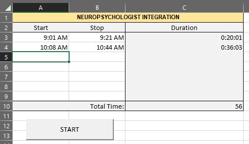
Example: Time tracking for billing.
- Create a table in Excel that includes columns for Start Time, End Time, and Duration.
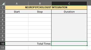
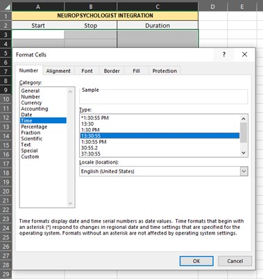
- Format the cells in the Start Time, End Time, and Duration columns so that they display times. Highlight the cells (A3:C9), right click, click on Format cells and change to “Time”.
- Add a formula to the Duration column to calculate the difference between the Start Time and End Time. For example, you could use the formula “=IF(AND(A3<>””,B3<>””),B3-A3,””)” (without the quotes ) in cell C3 to calculate the duration between cells A3 and B3.
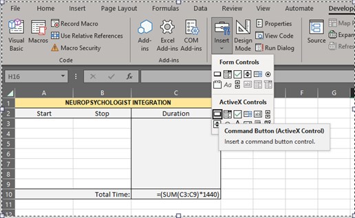
- Format cell C10 as “Number” and add a formula to calculate the total time (e.g., =SUM(C3:C9)*1440).
- Insert a Command Button. From the Developer tab, click “Insert” and add “Command Button”.
- Right-click on the Command Button and select “View Code.” This will take you to the Visual Basic Editor. Note: You can also click “Alt + F11” to open Visual Basic Editor, but using “right-click, view code” will take you to the command button’s code.
- In the Visual Basic Editor, you can write the code for the Command Button. There are many resources that will help with writing macro codes. I find that you can Google what you are interested in as well (e.g., “macro code for entering current time”). For example, you could use the code below to enter the current time in the Start Time or End Time column when the button is clicked:
Private Sub CommandButton1_Click()
If CommandButton1.Caption = "START" Then
CommandButton1.Caption = "STOP"
Dim q As Integer
For q = 3 To 9
If Cells(q, 1).Value = "" Then
Cells(q, 1).Value = Now()
Exit For
End If
Next q
Else
CommandButton1.Caption = "START"
Dim r As Integer
For r = 3 To 9
If Cells(r, 2).Value = "" Then
Cells(r, 2).Value = Now()
Exit For
End If
Next r
End If
End Sub
- The code enters the current time in the appropriate cell (A or B column) when the “Start/Stop” button is clicked. Cell C10 will keep a running total of the time you’ve spent on the given task.
You can use additional formulas to calculate the number of billable units (such as 96132/96133) based on the amount of time you spend on each task. There are a number of helpful resources online.
Helpful links:
https://support.microsoft.com/en-us/office/excel-video-training-9bc05390-e94c-46af-a5b3-d7c22f6990bb
https://www.excelfunctions.net/
Instagram: @exceldictionary and @thecheatsheets
https://formulabot.com/ for help with writing formulas and even VBA. Free account for non-profit organizations.
A list of functions in Excel can be found here: https://support.microsoft.com/en-us/office/excel-functions-alphabetical-b3944572-255d-4efb-bb96-c6d90033e188